Back-propagation learning in multi-layer networks

These notes have not yet been finalized for Winter, 1999.

Readings

Required readings: Chapter 9 except p265-275.

Learning as an optimization problem

The supervised learning problem can be posed as one of minimizing the sum of the squared errors between the output units' activations and the target activations. The problem is then how to adjust the weights in the network so as to minimize the total squared error. Minimizing a multi-dimensional function requires knowledge of introductory concepts from calculus.

Consider finding the minimum of the following function of two variables, starting at some random point:

We could do so by adjusting each of the two parameters in the direction that would move downhill along the surface of the function. This is the principal behind function minimization by gradient descent.

The general procedure is as follows:

For each pattern, compute the gradient (vector of partial derivatives) of the Error with respect to the weights.
Move each weight in the direction opposite to the corresponding component of the gradient; this is the direction of steepest descent.

If we adjust each variable in the opposite direction of the gradient, by a minute amount, we are guaranteed to decrease the function value.

The Delta Rule (also called the Widrow-Hoff or LMS rule)

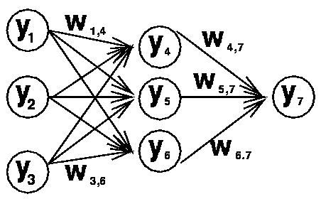
For linear networks, the outputs, y_i, are direct functions of the inputs, x_j, and the weights, W_ij:

The error measure to be minimized for supervised learning is:

and the learning rule for a particular weight W_ij to the ith unit is:

where epsilon is the learning rate, a small constant value.

Linear, multi-layer neural networks

Suppose we have the following multi-layer linear network:

If we define the weight matrix from the first to the second layer as W_1 and the weight matrix from the second to the third layer as W_2:

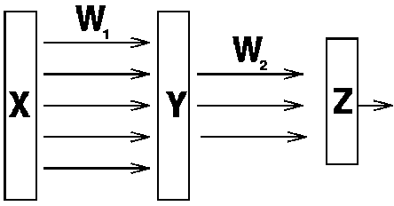
we can express the calculation performed by this network (i.e. the unit activations in each layer) as follows:

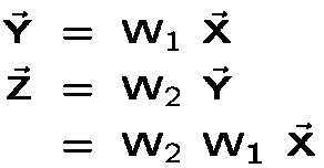
The product of two matrices, W_1 and W_2, is equal to a new matrix, W_3, so the above can be rewritten as:

Thus, a multi-layer linear network is shown to be equivalent to a single layer linear network with the weight matrices collapsed into one matrix. The extra layers don't buy us anything in terms of solving hard problems.

Adding a non-linearity

We need to make the unit activation functions non-linear to get extra power out of a multi-layer network. The most often used non-linearity is the sigmoid or logistic function:

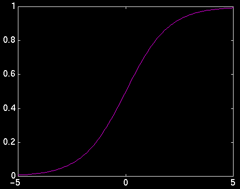
The derivative of the sigmoid function is:

This final form for the derivative is nice because it says that the derivative of the output of a unit with respect to its total input x can be expressed as a simple function of the unit's output f(x).

Delta rule for nonlinear units

When we add the nonlinearity, the error function is the same as for the linear delta rule, but the activation is computed differently and this affects the weight update equations. To simplify the derivation of the weight updates (particularly for the multi-layer case), we define an intermediary term delta which is the derivative of the error with respect to a unit's total input x. For an output unit i:

The back-propagation algorithm

For multi-layer networks, the deltas for the output layer are computed as above for non-linear units. For a unit j in the hidden layer, the delta term is computed as follows:

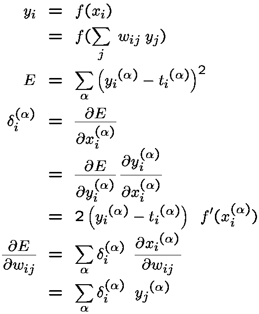
In the above equation, we have to sum over all output units i, because an incoming weight to a hidden unit j potentially affects the error of every output unit. So each hidden unit adds up the weighted sum of deltas being back-propagated along its outgoing connections to the output layer, multiplied by the weights on those connections. This weighted sum of deltas is then multiplied by the derivative of the sigmoid to get the hidden unit's own delta.

Once each unit (in any layer) has computed its own delta, it can obtain the weight update for each connection weight w_jk simply by multiplying the delta term by the incoming activation on that connection, y_k:

The back-propagation algorithm can be summarized as follows: For each training pattern, the network is activated and the target states are provided to the output units; for each output unit, the deltas are computed; for each hidden unit, the deltas are accumulated from the layer above to compute the hidden unit's delta; finally, for every unit in the network, the weight updates are computed.

If there is more than one hidden layer, each layer computes its deltas starting from the top layer down to the 2nd layer (one above the input layer). Once each layer's units have computed their deltas, they broadcast them by propagating them backwards on their incoming connections, multiplied by the incoming connection weights.

Theoretical results for multi-layer nonlinear networks

Neural networks are universal approximators Cybenko (1989): a neural network with non-linear hidden units, given a sufficiently large hidden layer, can approximate any continuous mapping (function) from inputs to outputs, to within any desired degree of accuracy.
Training a neural network may take longer than your lifetime: Judd (1988) and Blum & Rivest (1988) showed that for binary inputs and targets, the problem of finding a set of weights which would produce the correct mapping from input to target vectors (the loading problem) is NP-complete. The notion of NP-completeness is beyond the scope of the material presented here; however, suffice it to say that there exist worst-case mappings for which "it is unlikely that any algorithm which simply varies weights on a net of fixed size and topology can learn [the mapping] in polynomial time" (Baum, Neural Computation, 1988). To put it more simply, the number of learning iterations for back-propagation may be even worse than a polynomial function of the number of input units n, i.e. worse than n raised to any power you like, and maybe even be as bad as a scalar value raised to the power n.

Generalization, and the problem of over-fitting

To measure generalization performance, we divide the input patterns into two sets: a training set and a test set. The error on the training set tells us how well the network has learned to fit the data. The test set performance tells us how well the network generalizes. If the training set error is considerably lower than the test set error, we say that the network has over-fitted the data.

There are many heuristic solutions to the over-fitting problem, for example:

Weight decay: Minimize a cost function which combines the usual squared error with a penalty term which penalizes large weights (where lambda is a learning constant that determines the rate of weight shrinkage):

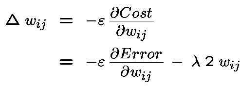
The learning rule now incorporates a weight shrinkage factor:
Weight constraints, for example, equality constraints as used in the le Cun et al digit recognition network (this will be covered in the next section on Applications).
Early stopping with cross-validation:Divide the training patterns into 3 subsets: a training set, a validation set and a test set. Train the network on the training set, but monitor its performance on both the training and validation set during learning. Stop training once the validation set error begins to rise (i.e., before over-fitting occurs).

Speeding up learning with momentum

An effective technique for accelerating learning is to allow the weight changes to build up momentum, becoming steadily larger for weights that are making steady progress in one direction, but not for weight changes that oscillate (e.g. increase, then decrease, then increase again) from one pattern to the next. Momentum is implemented as follows: (where alpha is another learning constant that defines the rate of momentum): Define a momentum matrix the same size as the gradient matrix for each layer, initialized to all zeros. Each time the gradient is calculated, increment the momentum matrix in proportion to (1 - alpha) times the previous value of momentum, plus alpha times the gradient. The weight update is then the learning rate times the momentum. A good value for alpha is between 0.9 and 0.95.

Check out the following demo of steepest descent with and without momentum on a quadratic surface:

quaddemo.m