The Perceptron Model
These notes have not yet been finalized for Winter, 1999.
Readings
Required reading: Chapter 8.
History of neural networks
- 1940's: Neural network models
- 1943, McCulloch & Pitts publish their paper "A Logical Calculus of the
IDeas Immanent in Nervous Activity" on their model neuron as a binary
threshold logic devic
- 1949, Hebb publishes his book "The Organization of Behavior" in which he
describes what is now known as "Hebbian cell assemblies"
- 1950's: Learning in neural networks
- the Hebbian learning rule
- 1951, Minsky publishes work on a Reinforcement learning machine
- 1960's: The age of the Perceptron (a period of massive enthusiasm)
- 1962 Rosenblatt published Principles of Neurodynamics, in which he
describes the Perceptron learning procedure
- Many wild claims are made by Rosenblatt and others about the potential
of Perceptrons as all-powerful learning devices
- 1970's: Limitations of Perceptrons are realized (the dark ages)
- 1969: Minsky and Papert's book "Perceptrons" is published, in which it
is shown that Perceptrons are only capable of learning a very limited class
of functions.
- Minsky & Papert predict that there will be no fruitful or interesting
extensions of Perceptrons even if multi-layer learning procedures are
developed
- The flow of funding into neural networks temporarily ceases
- 1980's: The discovery of back-propagation (the Renaissance)
- Back-propagation and other learning procedures for multi-layer neural
networks are invented
- The power of neural networks begins to be realized
- The hype cranks up again ...
Perceptrons
- The Perceptron learning procedure: an example of a supervised,
error-correcting learning procedure
- Perceptron convergence theorem
- Linearly separable problems: can be separated by a hyperplane
- Problems that are not linearly separable:
- XOR, connectedness
- any recognition problem that is invariant under a class of linear
transformations, e.g. translation-invariant pattern recognition
- Matlab demo
- encoding the thresholds as "bias weights" on an input line with a
constant activation of 1
- classification networks with linear threshold units can be viewed as
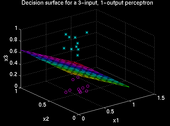
fitting a hyperplane to the decision boundary between classes (see figure below)
- Matlab code for a perceptron learning model:
 This graph shows the decision surface learned by the simple Perceptron defined
in the matlab code.
The surface is defined by the equation w1 x1 +
w1 x2 + w3 x3 + bias = 0, where the w's are the
weights and the x's are the inputs. The planar surface
indicates which input points (x1,x2,x3) will result in the
total input to the unit being zero, and it is orthogonal to the weight vector.
Points in the input space above this plane
will have a positive dot-product with the weight vector, and therefore cause the
unit to become active. Points in the input space below the surface will have a
negative dot product with the weight vector and therefore will not activate
the unit. Thus, this
critical region defines the classification boundary learned by the perceptron.
For the linearly separable data set shown in the graph, the perceptron was
able to classify the data perfectly.
![[Previous]](prevsec.gif)
![[Parent]](parntsec.gif)
![[Next]](nextsec.gif)