Hopfield networks and Boltzmann machines

Section on Boltzmann machines will not be covered in 1999.

Readings

Required readings: Chapter 12 and sections 10.1 and 10.8 in coursepack article "Neural network approaches to solving hard problems". In 1999, we will only cover the sections in chapter 12 up to page 413.

Definition of a Binary Hopfield Network

The standard binary Hopfield network is a recurrently connected network with the following features:

symmetrical connections: if there is a connection going from unit j to unit i having a connection weight equal to W_ij then there is also a connection going from unit i to unit j with an equal weight.
linear threshold activation: if the total weighted summed input (dot product of input and weights) to a unit is greater than or equal to zero, its state is set to 1, otherwise it is -1. Normally, the threshold is zero. Note that the Hopfield network for the travelling salesman problem (assignment 3) behaved slightly differently from this.
asynchronous state updates: units are visited in random order and updated according to the above linear threshold rule.
Energy function: it can be shown that the above state dynamics minimizes an energy function.
Hebbian learning

The most important features of the Hopfield network are:

Energy minimization during state updates guarantees that it will converge to a stable attractor.
The learning (weight updates) also minimizes energy; therefore, the training patterns will become stable attractors (provided the capacity has not been exceeded).

However, there are some serious drawbacks to Hopfield networks:

Capacity is only about .15 N, where N is the number of units.
Local energy minima may occur, and the network may therefore get stuck in very poor (high Energy) states which do not satisfy the "constraints" imposed by the weights very well at all. These local minima are referred to as spurious attractors if they are stable attractors which are not part of the training set. Often, they are blends of two or more training patterns.

The Boltzmann machine, described below, was designed to overcome these limitations.

Hopfield network demo

The following matlab program sets up a Hopfield network having units arranged in a 2-dimensional grid with local connectivity. Each unit is symmetrically connected to its four nearest neighbors on the grid and the connection weights are all equal to 1.0. This example is described further in Anderson, Chapter 12. To achieve a minimum in energy, every unit should agree with its four neighbors. Thus, all units should be in the same state to achieve a mininum energy configuration.

The states of the units in the network are initialized as follows: a central square of units are turned on, the rest are turned off, and then all units are randomly flipped with probability 0.1.

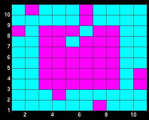Here is an example of the initial state of the network.

For this network, there are only two global energy minima, one with all units on and one with all units off. After settling, however, the network usually ends up in a "blend state" which is a blend of the two global minima.

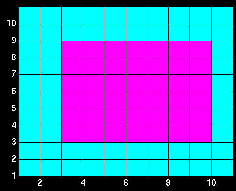Here is an example of the final state of the network after settling. This is a local minimum, sometimes called a spurious attractor.

Matlab code:

initHopfield.m (initialization module)
forwardHopfield.m (state updates)
scramble.m (function)
plotHopActivations.m
init2Dweights.m (function)

You can run the above demo by loading initHopfield, and then repeatedly loading forwardHopfield. Each time forwardHopfield is run, you should then call plotHopActivations, to display the states of all units in the network in a 2-dimensional layout.

Boltzmann Machines

The binary Boltzmann machine is very similar to the binary Hopfield network, with the addition of three features:

Stochastic activation function: the state a unit is in is probabilistically related to its Energy gap. The bigger the energy gap between its current state and the opposite state, the more likely the unit will flip states.
Temperature and simulated annealing: the probability that a unit is on is computed according to a sigmoid function of its total weighted summed input divided by T. If T is large, the network behaves very randomly. T is gradually reduced and at each value of T, all the units' states are updated. Eventually, at the lowest T, units are behaving less randomly and more like binary threshold units.
Contrastive Hebbian Learning: A Boltzmann machine is trained in two phases, "clamped" and "unclamped". It can be trained either in supervised or unsupervised mode. Only the supervised mode was discussed in class; this type of training proceeds as follows, for each training pattern:
1. Clamped Phase: The input units' states are clamped to (set and not permitted to change from) the training pattern, and the output units' states are clamped to the target vector. All other units' states are initialized randomly, and are then permitted to update until they reach "equilibrium" (simulated annealing). Then Hebbian learning is applied.
2. Unclamped Phase: The input units' states are clamped to the training pattern. All other units' states (both hidden and output) are initialized randomly, and are then permitted to update until they reach "equilibrium". Then anti-Hebbian learning (Hebbian learning with a negative sign) is applied.
The above two-phase learning rule must be applied for each training pattern, and for a great many iterations through the whole training set. Eventually, the output units' states should become identical in the clamped and unclamped phases, and so the two learning rules exactly cancel one another. Thus, at the point when the network is always producing the correct responses, the learning procedure naturally converges and all weight updates approach zero.
The stochasticity enables the Boltzmann machine to overcome the problem of getting stuck in local energy minima, while the contrastive Hebb rule allows the network to be trained with hidden features and thus overcomes the capacity limitations of the Hopfield network. However, in practice, learning in the Boltzmann machine is hopelessly slow.

In class, we saw a demonstration on overhead transparencies of the Boltzmann machine performing figure-ground segregation. This network was hard-wired (i.e. hand-selected weights, no learning). Some units were designated as "edge units" which had a particular direction and orientation, while others were designated as "figure-ground units". At each image location there was a full set of edge units in every possible orientation (horizontal or vertical) and direction (left, right, up or down), and a full set of figure/ground units (one of each). The weights could be excitatory or inhibitory, and represented particular constraints amongst the figure/ground and edge units. For example, an edge unit at one location would inhibit the edge unit of the same orientation but opposite direction at the same location. Another example: a vertical right-ward pointing edge unit would excite a figure unit at the next image local to the right, and inhibit a ground unit at that location, and would inhibit the figure unit to the left and excite the ground unit to the left. The entire network was initialized with the appropriate edge units turned on, and all other units off, and then all units were randomly flipped with some small probability so that the input was noisy. Units states were then updated using simulated annealing. The network was shown to be able to fill in continuous regions and label them as either figure or ground. The region could be non-convex (e.g. the letter C). The network could also fill in non-continuous edges, exhibiting "illusory contours".